 ControlHub
Pendulim Platform
The rotary inverted pendulum is an academic experimental setup for prototyping of feedback control algorithms. The pendulum platform of ControlHub is based on QUBE - Servo 2 from Quanser. The access to the pendulum experiment server is here (presently available only in the local network of Inria Lille due to security reasons)

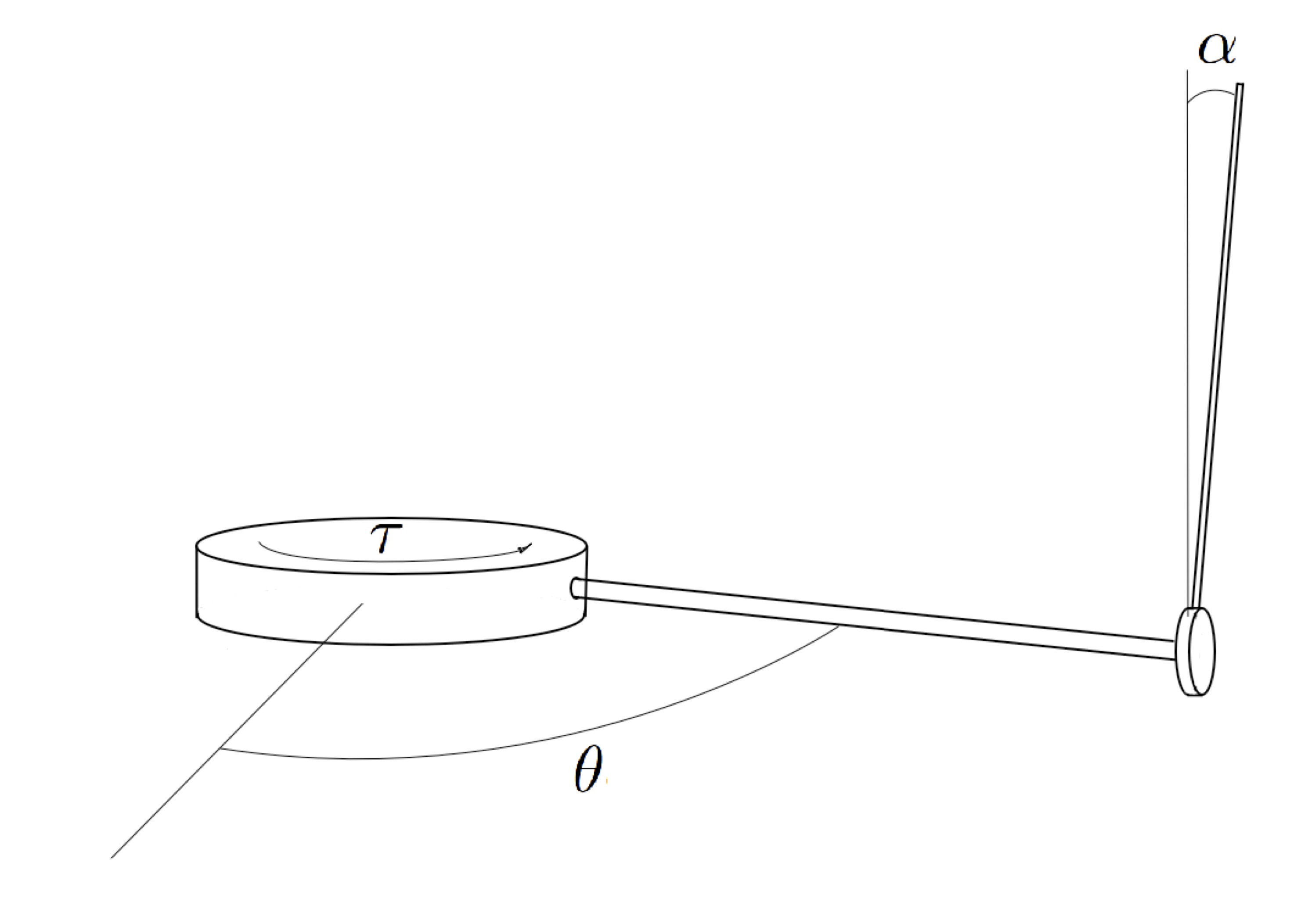
A schematic representation of the rotary inverted pendulum (IP), also known as Furuta Pendulum, is shown on the above figure. This is a two-link mechanical system. The first link is the rotary arm rigidly connected on the one side to a rotor of an electrical motor being an actuator of the system. The second link is the pendulum installed at the other side of the rotary to the rotary arm. The pendulum's motion is possible only in the plane orthogonal to the rotary arm. The generalized coordinates $\theta$ and $\alpha$ describe the angular positions of the rotary arm and the pendulum, respectively. To obtain motion equations, the pendulum is considered as a lumped mass at its center.
Mathematical model
The following table presents the notation utilized for model description.| $\textbf{Symbol} $ | $\textbf{Description}$ |
|---|---|
| $\alpha$ | Angle of the pendulum arm |
| $\theta$ | Angle of the rotary arm |
| $m_p$ | Mass of the pendulum |
| $L_p$ | Length of the pendulum |
| $J_p$ | Inertia of the pendulum |
| $D_p$ | Pendulum damping coefficient |
| $L_r$ | Length of the rotary arm |
| $J_r$ | Rotary arm inertia |
| $D_r$ | Viscous damping coefficient |
| $g$ | Gravitation constant |
| $\tau$ | Torque of servo motor |
Control System
Model is given by the equation (3)Control input: $V_m$ - the input voltage to the servo motor
Measured output: $\alpha$ - the angle of the pendulum arm and $\theta$ - the angle of the pendulum arm
Control Tasks
Problem 1 (Stabilization): Regulate $\alpha(t) \to 0$ (upper position) and $\theta(t)\to 0$Problem 2 (Setpoint tracking): Regulate $\alpha(t) \to 0$ (upper position) and $\theta(t)\to\mathrm{step}(t)$ (a step function with several levels)
Problem 3 (Trajectory tracking): Regulate $\alpha(t) \to 0$ (upper position) and $\theta(t)\to \theta^*(t)$ (a smooth desired reference function)
Control Research with Experiments on Pendulum Platform of ControlHub
- D. Cruz-Ortiz, M. Ballesteros, A. Polyakov, D. Efimov, I. Chairez, A. Poznyak, Practical Realization of Implicit Homogeneous Controllers for Linearized Systems, IEEE Transactions on Industrial Electronics, 2021 (hal)
- G. Perozzi, A. Polyakov, F. Miranda-Villatoro, B. Brogliato, Upgrading linear to sliding mode feedback algorithm for a digital controller, IEEE Conference on Decision and Control, 2021 (hal)
- G. Perozzi, A. Polyakov, F. Miranda-Villatoro, B. Brogliato, Upgrading a linear controller to a sliding mode one: Theory and experiments, Control Engineering Practice, 2022 (hal)
- S. Wang, H. Duan, G. Zheng, X. Ping, D. Boutat, A. Polyakov, Homogeneous control design using invariant ellipsoid method, IEEE Transactions on Automatic Control, 2024 (hal)
- D. Efimov, A. Polyakov, Contrôle et estimation à temps fixe ou fini, Techniques de L'ingenieur, 2024, Réf : S7442